Uncertainty Propagation

The goal of this library is to provide an tool to experimentalists in the field of shock-wave compression experiments to predict the outcome of in an expedited manner. Until now, detailed Hydrocode software simulations that involved the whole Equation of State (EOS) of materials are used, to predict the way a shock propagate through a sequence of materials, thus replicating an experiment. This computationally expensive process can only replicate a small range of initial conditions within a short time-frame while it does not account introduced errors, such deviations of the laser drive, regions of EOS with limited results, etc.

These exact shortcomings is what the proposed library is trying to address, and provide a complimentary tool that can reproduce the experiment in expedited manner while taking account the intrinsic uncertainties of the EOS and input measurements.

At the same time, multiple sources of uncertainty can be taken into account, such as uncertain input pressure of the experiment, uncertain material EOS, represented by its uncertain Hugoniots. All the above can provide experimentalists with both an estimation of the final experimental results, as well as uncertainty measures in the form of distributions and statistical moments of predicted final locus of predictions.

At the same time, a common practice for post-processing the results after an experiment, is to use the measured quantities at the window layer and employ the Impedance Matching technique to infer the EOS of the sample material under study. This backward propagation of an experiment has also been implemented in this framework, as a way to support the experimentalist tools while providing measures of uncertainties.

Forward Experiment Propagation

Shock-wave Experiment Class

Methods

class ShockWaveExperiment(materials: list[Material])

Class simulating the forward propagation of experiment using the same sequence of materials as in the experimental setup.

Parameters:

materials – A list containing Material objects in the same sequence as in the experiment.

run_experiment(shock_pressure: float, cov=None, initial_points: int = 500, n_isentropes_per_material: int | None = None)

Upon initialization of the class, this method is used to forward propagate the experiment using the Impedance Matching technique.

Parameters:

• shock_pressure – Predefined pressure of the input laser drive.

• cov – Coefficient of variation of pressure assumed for the laser drive. If value of this parameter is None, the algorithm will assume there is no uncertainty in the input.

• initial_points – This parameter defines the number of points to be drawn from a Normal distribution with mean value the shock_pressure and standard deviation inferred using the cov parameter. This will create a number of initial shocked states where the experiment will start from, thus taking into account the uncertainty of the input laser drive.

• n_isentropes_per_material – This parameter limits the number of isentropes generated and propagated from one material to the next, and as a result prevents the number of experiment evaluations from growing geometrically.

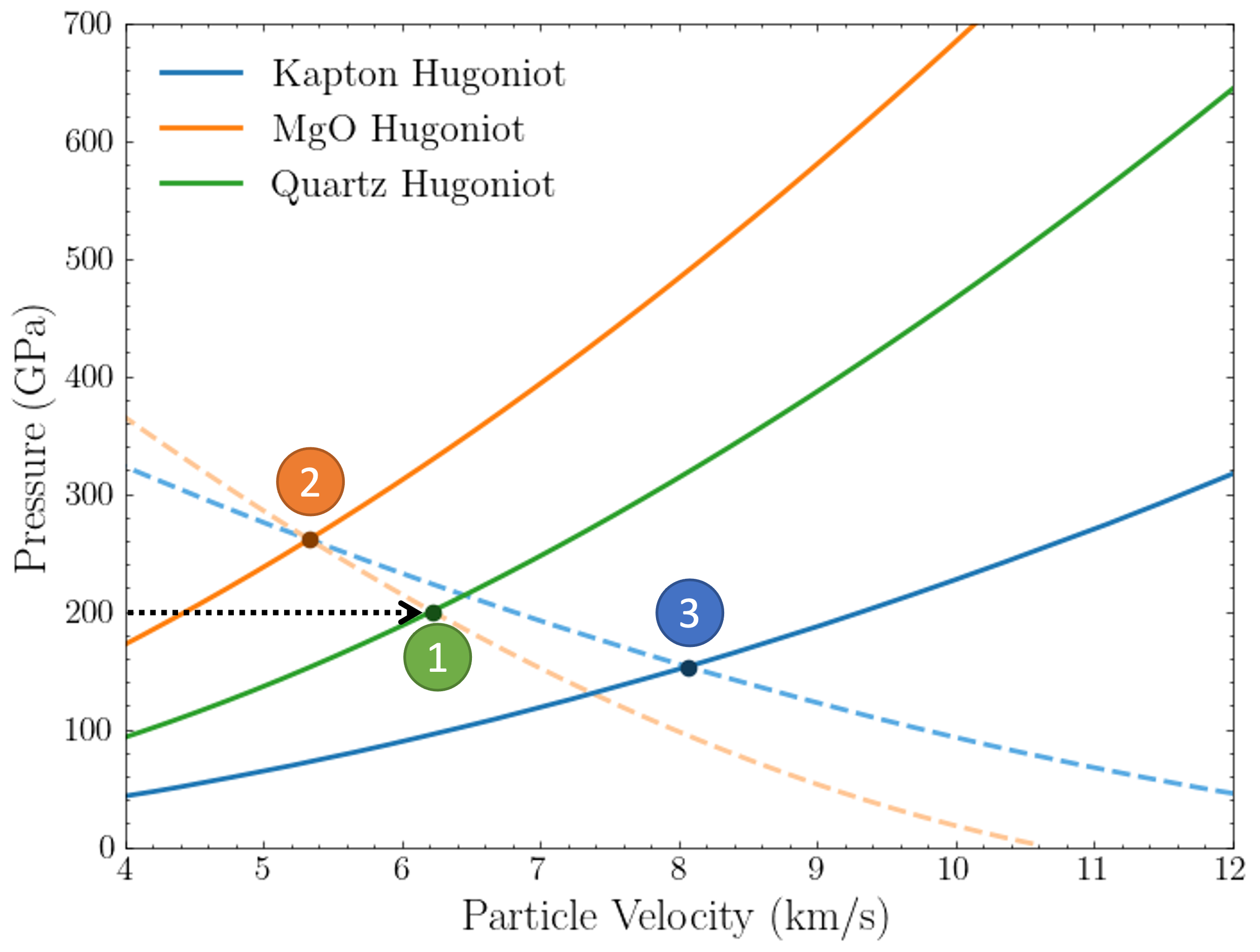
plot()

This functions plots all possible experimental paths the forward propagation of an experiment has taken into account, creating a plot similar to the one below.

Backward Experiment Propagation

Backward Shock-wave Experiment Class

Methods

class BackwardPropagationFromWindow(materials: list[Material])

Class simulating the backward propagation of experiment using the same sequence of materials as in the experimental setup.

Parameters:

materials – A list containing Material objects in the same sequence as in the experiment.

propagate(measured_pressure: float, cov=None, initial_points=1000, n_intersections_per_material: int | None = None)

Upon initialization of the class, this method is used to backward tracethe experiment using the Impedance Matching technique.

Parameters:

• measured_pressure – Pressure measure at the window material layer of the experimental setup.

• cov – Coefficient of variation of pressure measured at the window layer. If value of this parameter is None, the algorithm will assume there is no uncertainty in the measurement.

• initial_points – This parameter defines the number of points to be drawn from a Normal distribution with mean value the measured_pressure and standard deviation inferred using the cov parameter. This will create a number of initial measured pressures where the experiment will start from, thus taking into account the uncertainty of the window measurement.

• n_intersections_per_material – This parameter limits the number of shocked states calculated during the backward propagation of the experiment, and as a result prevents the number of experiment evaluations from growing geometrically.

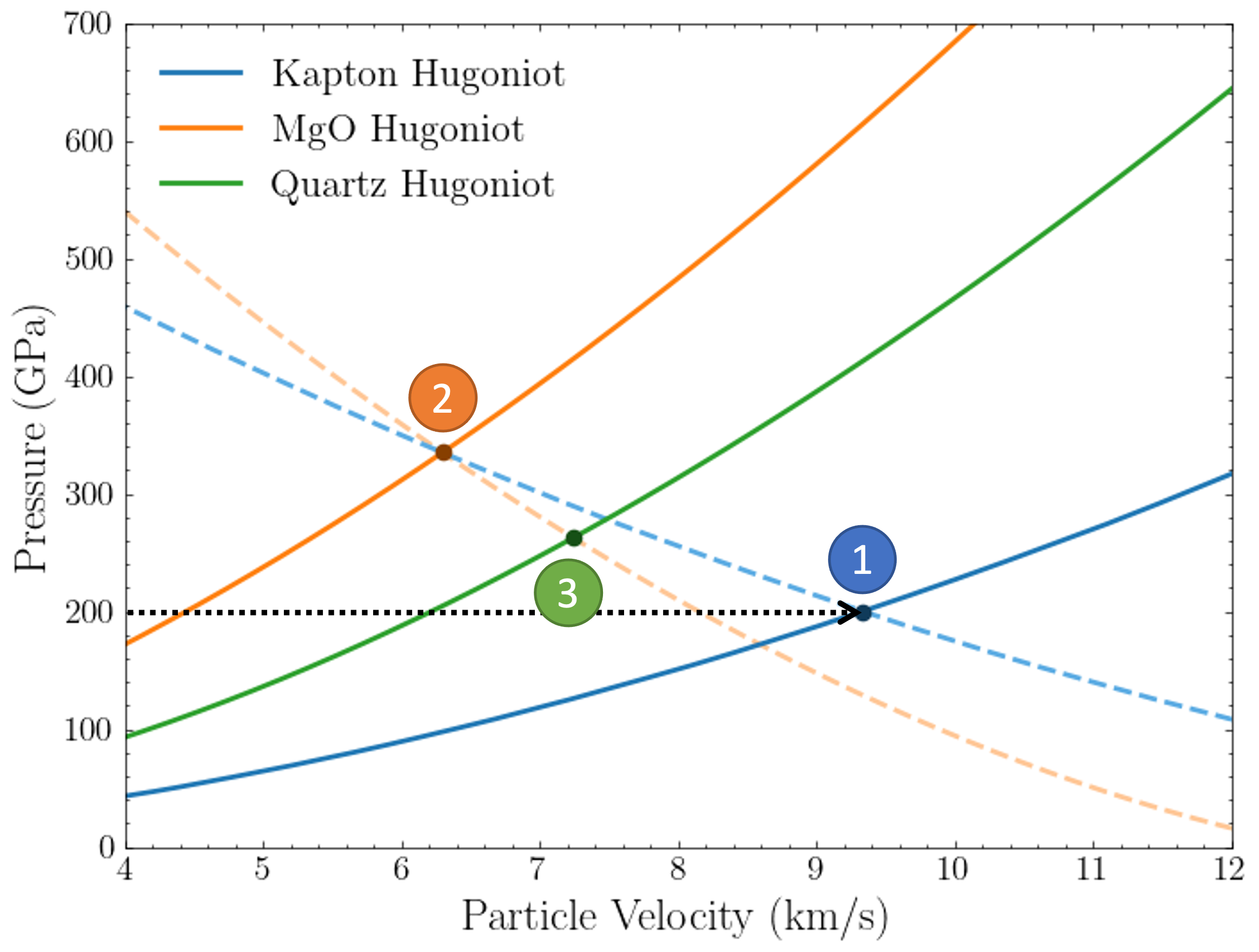
plot()

This functions plots all possible experimental paths the backward propagation of an experiment has taken into account, creating a plot similar to the one below.

Examples

• Shock-wave experiment examples